Guide to Adjusting Trading Strategies Based on Volatility
Introduction
This guide helps traders adjust their trading strategies based on market volatility, specifically the Time Warp strategy and Batman configurations. By understanding the volatility regime (big picture) and local implied volatility (IV) (daily picture), you can optimize your trades and manage risks effectively.
Understanding the Basics
Market Influences:
- Economic Reports: Employment data, GDP reports, inflation figures, etc.
- Geopolitical Events: International conflicts, policy changes, elections, etc.
- Earnings Announcements: Quarterly reports, forecasts, company news, etc.
- Significant Events: Major industry news, unexpected events, natural disasters, etc.
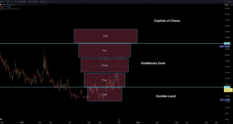
Volatility Regime (Big Picture):
- Zombieland (VIX Below 17): Characterized by low volatility and stable market conditions.
- Goldilocks Zone (VIX Between 17-32): Moderate volatility, balanced market conditions.
- Chaos Zone (VIX Above 32): High volatility, unstable market conditions.
Local Implied Volatility (Daily Picture):
- Daily fluctuations in IV are influenced by immediate market events.
- Requires constant monitoring to adjust trading strategies accordingly.
Adjusting Strategy Characteristics
1) Number of Days Out (Time Warp Strategy):
Zombieland (VIX Below 17):
- Days to Expiration (DTE): Use multiple DTE strategies (1, 2, or 3 DTE) to capture limited price movements and premium decay over several days.
- Overnight Market Moves: The Time Warp strategy is particularly useful when a significant percentage of market moves occur in the overnight session, resulting in small doji days. This allows traders to recapture directional moves they would normally miss in a 0-DTE trade.
- Infrequent Usage: This strategy adjustment is not used often and is used only in low volatility situations with unusual overnight gap situations.
- Example: When VIX is around 12-13, consider placing trades with 1-3 DTE to account for the low volatility environment and overnight market moves.
Goldilocks Zone (VIX Between 17-32):
- Days to Expiration (DTE): Focus on shorter DTE (0-DTE to 2-DTE) to take advantage of moderate volatility and quicker premium decay.
- Example: If VIX is around 20-25, use 0-2 DTE trades to benefit from the balanced market conditions.
Chaos Zone (VIX Above 32):
- Days to Expiration (DTE): Primarily use 0-DTE trades to manage the high volatility and capture rapid premium decay.
- Example: With VIX above 32, deploy 0-DTE trades to effectively navigate the high volatility environment.
2) Using the Batman Strategy:
Zombieland (VIX Below 17):
- Batman Strategy: Generally not used in low volatility environments due to limited price movements.
- Example: Avoid Batman configurations when VIX is below 17; focus on narrower butterfly spreads.
Goldilocks Zone (VIX Between 17-32):
- Batman Strategy: Effective in this range, offering a balance between risk and reward.
- Risk-to-Reward Ratios: Use varying ratios (30-70%, 40-60%, 70-30%) based on specific VIX levels.
- Percentage of Time: The Batman strategies range (e.g., 40-60%) indicates the percentage of time you choose between a single OTM fly and a Batman configuration.
- Example: If VIX is around 25, you might choose Batman configurations 40% of the time and a single OTM fly 60% of the time for better risk management.
Chaos Zone (VIX Above 32):
- Batman Strategy: Highly effective, providing wide spreads to handle significant price movements.
- Risk-to-Reward Ratios: Use wider ratios (e.g., 30-70%) to accommodate the higher volatility.
- Percentage of Time: Adjust the frequency of using Batman configurations versus single OTM flies based on the specific VIX level.
- Example: With VIX above 32, deploy Batman configurations with appropriate risk-to-reward ratios to manage increased market risk and use them more often.
Monitoring and Adapting
Monitor Local IV:
- Use real-time data and alerts to track daily IV changes.
- Adjust the number of DTE and strategy configurations based on significant IV shifts.
Adapting to Daily Influences:
- If a daily economic report or event causes a notable IV spike, immediately adjust your strategy.
- Example: If VIX jumps from 12 to 15 due to a weak employment report, adjust from multiple DTE trades to single DTE trades with wider butterfly spreads.
Continuous Learning:
- Stay informed about market conditions and upcoming events.
- Engage with the trading community to share insights and strategies.
Conclusion
Adapting your trading strategies, such as the Time Warp strategy and Batman configurations, based on the volatility regime and local IV is crucial for managing risk and maximizing returns.
Following this guide, you can better navigate different market conditions and enhance your trading performance.